Assessing Pay for Performance

Although pay for performance is a nearly universal objective of executive compensation programs, there is little agreement on how to measure it and monitor it. Companies often seem to believe that it is obvious that pay varies with performance, while many investors feel that there is little evidence of a strong correlation between the two. This report explores five interpretations of the “pay for performance” concept, presents a practical way to measure it, assesses the concept’s prevalence, and explains how directors can monitor and improve pay for performance at their company.

Five Interpretations of “Pay for Performance”

An analysis of “pay for performance,” as used by the business community, reveals that there are at least five interpretations of the concept.

1. Pay versus target pay is tied to performance Many companies believe that they achieve pay for performance because they award compensation that is above a target level when performance is good and below a target level when performance is poor. For example, in its 2010 proxy statement, Procter & Gamble describes pay for performance this way: “We pay above target when goals are exceeded and below target when goals are not met.” [1] However, few institutional investors and proxy voting advisors are comfortable with a pay for performance concept tied to target pay levels, as they believe that, under this construct, some companies may adopt needlessly high target pay levels and reward poorly performing executives with pay levels that, albeit lower than those for well-performing executives, remain above the market.

2. Pay doesn’t go up when performance is poor Institutional Shareholder Services (ISS), a leading proxy voting advisor, has tried to get away from target levels by defining pay for performance in terms of performance and pay changes. In its 2008 U.S. proxy voting guidelines, ISS said it would vote against compensation committee members when “the company has a pay-for-performance disconnect,” defined as an increase in pay coupled with a decrease in performance. [2] An obvious weakness of this approach is that it makes no distinction between poorly performing CEOs who are paid well below the market and those who are paid well above it.

3. Pay versus market pay is tied to performance The shortcomings of using target pay or prior year pay as a benchmark for assessing pay for performance has led some companies to focus instead on market pay. Dow Chemical says it “believes in pay-for-performance…. We target all elements of our compensation programs to provide compensation opportunity at the median of our peer group. Actual payouts under these programs can be above or below the median based on Company and personal performance.” [3] CSX Corporation says its “objective is to provide total pay opportunities that are competitive with those provided by peer companies in the railroad industry and general industry, with actual payment dependent upon performance.” [4] Both Dow Chemical and CSX agree that superior performance should lead to above market pay and poor performance should lead to below market pay, but neither company says how much total compensation should differ from market pay for any level of outperformance, nor discloses its market pay estimates.

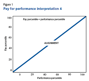4. Pay percentile = performance percentile The Conference Board Task Force on Executive Compensation articulated a specific target relationship between outperformance and above market pay: a company’s pay percentile should equal its performance percentile. Its 2009 report states, “If a company provides target levels of pay at or above a particular percentile and does not perform at that percentile of peer companies on a sustained basis, the company should redesign its compensation strategy to align it with the organization’s performance.” [5] Compensation consulting firm Pay Governance takes a similar position. It argues that “by comparing a company’s Realizable Pay percentile to its performance percentile for the same time period, it is possible to see how well a company’s pay and performance was aligned….. if realizable pay is well above-median with below-median performance… this indicates poor alignment in the pay program.” [6] This view can be summarized in a simple graph (see Figure 1), where the vertical axis is pay percentile and the horizontal axis is performance percentile.

Pay for performance is the main diagonal where pay percentile equals performance percentile. The only reason to grant above-market pay is superior performance.

5. Pay for performance has three dimensions: incentive strength, cost control, and alignment A fifth interpretation is that pay for performance has three dimensions:

• the sensitivity of relative pay to relative performance;
• the pay premium, if any, at industry-average performance, and
• the correlation of relative pay and relative performance

This view of pay for performance can also be summarized in a simple graph, where the vertical axis is relative pay and the horizontal axis is relative performance and we draw the regression trendline (i.e. the line of “best fit”) between relative pay and relative performance (see Chart 10). In this graph, the slope of the line shows the sensitivity of relative pay to relative performance (or pay leverage)—that is, the ratio of percent change in relative pay to percent change in relative performance. The intercept shows the pay premium for industry-average performance, a measure of cost control. The correlation offers a measure of alignment or design efficiency for the compensation program. When the correlation is high (and positive), there is little pay that is unrelated to performance.

Under this view of pay for performance, each company must decide what the appropriate pay leverage is. One possible answer is interpretation #4 (i.e., that the appropriate pay leverage is the one resulting from the application of the principle “pay percentile equals performance percentile”). However, this may not be the right answer for many companies. In fact, as discussed later, this pay leverage is higher than the leverage actually achieved by 95 percent of S&P 1500 companies and there is wide variation in pay leverage among companies. There may also be wide variation in optimal pay leverage among companies. This interpretation of the pay-for- performance concept does not require average pay for industry-average performance, but it does suggest that the likely justification for a pay premium is an above-average incentive—that is, an above-average pay leverage.

Four Measures of Pay

Both The Conference Board Task Force on Executive Compensation and Pay Governance endorse the concept that “pay percentile equals performance percentile.” However, they apply it to different measures of pay. Specifically, The Conference Board Task Force applies the concept to “target pay,” while Pay Governance applies it to “realizable pay.”

1. Target pay Target pay is a measure of the “expected value” of compensation at the start of the year or the date of grant. Target pay includes salary, target cash bonus, and target equity compensation. Target equity compensation may be a stated dollar amount (e.g., $2 million) or a stated dollar equivalent amount (e.g., 100 percent of salary). If a company doesn’t have a formal policy, target equity compensation is the expected value of the year’s equity compensation at the date of grant.

In all of these cases, target pay refers to the expected value of equity compensation before or at the date of grant and does not include changes in the value of the stock or option after the date of grant. Another term for target pay—used by Dow Chemical in its 2010 proxy—is “compensation opportunity.”

2. Mark-to-market (realizable) pay Realizable pay is an effort to develop a pay measure that captures the incentives provided by changes in the value of unvested stock and unexercised options as well as by the difference between actual and target bonus.

Realizable pay for a three-year period is the sum of:

• Salary, annual bonus, and “other” compensation during the three years.
• The end-of-period value of equity compensation granted during the three-year period
  • Equity compensation includes stock options, performance shares, and restricted stock.
  • The value of a stock option grant is based on the Black-Scholes model using the stock price at the end of the three-year period.
  • The value of a performance share grant is based on the number of shares expected to vest and the stock price at the end of the three year period.
• The end-of-period value of cash long-term incentive awards made during the three-year period, and
• The change in pension value over the three-year period.

It is not strictly “realizable” pay because unvested equity compensation is included. In this report, the term “mark to market pay” is used in lieu of “realizable pay” because the pay value includes unvested equity compensation that is not currently realizable.

3. Proxy statement pay The total compensation figure reported to investors in the Summary Compensation Table of proxy statements falls in between target pay and mark-to-market pay. It differs from target pay because it includes actual cash bonus, not target bonus, and actual equity compensation grants, not the target equity compensation grant value. It also includes the grant-date expected value of equity compensation, not the value based on the end of period stock price.

4. Grant-date pay This report uses a measure called “grant-date pay,” a modified version of proxy-statement pay that provides a better approximation of a company’s target compensation. It differs from the proxy statement total compensation figure because it includes:

• the full expected value of equity compensation grants made in the year, not the accounting allocations used in the Summary Compensation Table [7] ;
• the expected value of non-equity incentive compensation, not the actual non-equity incentive award in the year; and
• the expected return on the executive’s beginning of year pension value, not the actual change in pension value during the year.

The Importance of Value Leverage

The concept that pay percentile should equal performance percentile is fairly easy to understand. However, it is impossible to design a pay program that achieves that result without translating this pay-for-performance concept into “value leverage,” which is the ratio of percent change in pay to percent change in performance. To demonstrate the importance of value leverage, consider the ability of a simple stock compensation plan to achieve “pay percentile equals performance percentile.”

Chart 1 shows the distribution of three-year mark-to-market pay, expressed as a multiple of three-year grant-date “market pay” for CEOs in the Execucomp database. Grant-date market pay is the trendline value of grant-date total compensation for an executive’s position, industry, and company revenue size.

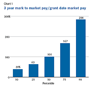We will assume that the CEO’s sole compensation for the three-year period is a single up-front performance stock grant, that grant-date market pay is $1 million per year, and that the expected return on the stock is 10 percent. Since the expected Year 3 value of the stock is 133 percent of the grant-date value, an up-front stock grant of $2.25 million will provide a Year 3 expected value of $3 million. We will use the percentages from Chart 1 to calculate vesting percentages: 39 percent at the 10th percentile total shareholder return (TSR), 63 percent at the 25th percentile TSR, 101 percent at the 50th percentile TSR, 167 percent at the 75th percentile TSR, and 284 percent at the 90th percentile TSR.

Mark-to-market pay and grant-date market pay For simplicity, assume that 50th percentile performance is equal to expected performance. If the 50th percentile performance is achieved, the vesting percentage is 101 percent, the market value of the initial grant shares is $3.00 million, and mark-to-market pay (i.e., the year 3 value of the vesting shares) is $3.03 million. This structure accomplishes a 50th percentile pay for 50th percentile performance.

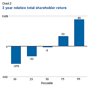
Now assume that 25th percentile performance is achieved. With an initial stock price of $10 and an original grant of 225,000 shares, the number of shares vesting at the 25th percentile performance will be 63 percent x 225,000 = 142,000. Since the stock value at the 50th percentile is $13.30 (i.e., $10 x 133 percent), the stock value at the 25th percentile will be less. Chart 2 shows that the three-year stock value at the 25th percentile performance is, on average, about 29 percent less than at the 50th percentile. The stock value is likely to be $9.44, and the aggregate stock value is $1.34 million (142,000 x $9.44), or 45 percent of the grant-date market pay. As a result, the mark-to-market pay value is close to the 10th percentile when performance is at the 25th percentile.

This analysis shows that the proposed simple compensation plan overshoots the pay objective on the downside because the pay percentile is less than the performance percentile.

A similar problem occurs if 75th percentile performance is achieved. The number of shares vesting will be 376,000 (167 percent x 225,000). The stock value at the 75th percentile performance is, on average, about 36 percent more than at the 50th percentile. The stock value is likely to be $18.09. As a result, the aggregate stock value is $6.8 million (376,000 x $18.09), or 227 percent of the grant-date market pay. This produces a mark-to-market pay value closer to the 90th percentile. In this case, the proposed simple compensation plan overshoots the pay objective on the upside because the pay percentile is greater than the performance percentile.

The proposed simple compensation plan is too leveraged: it declines too much for poor performance and rises too much for good performance. The problem is that its vesting schedule is based directly on the pay distribution and, as a result, captures the full variation in mark-to-market pay. When the leverage in the vesting percentage is combined with the leverage in the stock value, the variation in mark-to-market pay is overshot.

To design a plan that achieves the “pay percentile equals performance percentile” paradigm, it is necessary to understand the value leverage implied by that principle. If the principle implies that a 10 percent change in relative shareholder value increases mark-to-market pay by 15 percent, the vesting schedule can be calibrated so that the combined effect of vesting schedule leverage and stock value leverage is equal to the target leverage. If the vesting percentage increases by 5 percent when relative shareholder value increases by 10 percent, the combined effect will be 15 percent.

Estimating Pay Value Leverage

Pay “value leverage” is the ratio of percent change in relative pay to percent change in relative performance. We first estimate pay leverage under the assumption that pay percentile is equal to performance percentile. We then estimate average pay leverage in the labor market and the range of individual company pay leverage.

Relative pay Relative pay is actual pay divided by market pay. Actual pay is mark-to-market pay for a three-year period. Market pay is average mark–to-market pay taking account of each executive’s position, industry, and company revenue size. [8] We have developed market rates for the top-five executives reported in S&P’s Execucomp database for the three year periods ending in 1995-2009. We exclude three-year periods in which an executive is promoted to CEO. The market rate models are done separately for each three-year period and for each of the 24 GICS (i.e., the Global Industry Classification Standard developed by Standard & Poor’s and Morgan Stanley International) industry groups, giving a total of 360 market pay models. [9]

To estimate pay leverage under the assumption that pay percentile is equal to performance percentile, we calculate the distribution of relative pay for all the cases in our sample, a total of 63,936 cases (each case is one executive for one three year period). We use a log measure of relative pay, consistent with the log models that have been used to model pay-size relationships for more than 50 years. [10] Log differences, unlike simple percentage differences, are additive. [11]

The distribution of relative pay shows, for example, that log relative pay is -0.45 at the 25th percentile and +0.39 at the 75th percentile. This means that the 25th percentile executive had a three-year mark-to-market pay 36 percent below the average for his or her position, industry and company size, while the 75th percentile executive had a three-year mark-to-market pay 48 percent above average for the individual’s position and industry. [12]

Relative performance Relative performance is actual shareholder wealth divided by shareholder wealth assuming the industry average return. We use a log measure of relative performance, just as we do for relative pay. [13] Log relative performance is -0.36 at the 25th percentile and +0.30 at the 75th percentile, meaning that the 25th percentile executive/company had a three-year TSR 30 percent below the industry return, while the 75th percentile executive/ company had a three-year TSR 35 percent above the industry return.

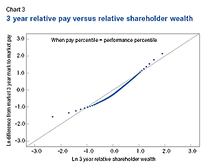
Plot relative pay and relative shareholder wealth for each percentile Chart 3 shows relative pay and relative shareholder wealth for each percentile. The vertical axis is log relative pay, while the horizontal axis is log relative shareholder wealth. Each plot point represents one percentile. The dashed line on the main diagonal has a slope of 1.0, and hence, shows where pay value leverage is 1.0. On this line, the change in log relative pay is exactly equal to the change in log relative shareholder wealth.

The graph shows that pay leverage for superior performance is greater than pay leverage for poor performance. When relative TSR is positive, the plot point line is steeper than the main diagonal, meaning that pay leverage is greater than 1.0. When relative TSR is negative, the plot point line is less steep than the main diagonal, meaning that pay leverage is less than 1.0.

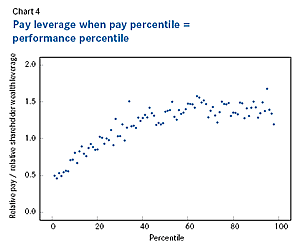
Calculate pay leverage at each percentile We can calculate the pay leverage at each percentile (i.e., the ratio of the log percent change in relative pay to the log percent change in relative shareholder wealth). [14] Chart 4 shows a scatterplot of pay leverage on the vertical axis against pay and performance percentile on the horizontal axis.

Pay leverage increases from about 0.4 at the first percentile to about 1.4 at about the 50th percentile. Up to the 50th percentile, the trendline formula for leverage is 0.52 + .018 x percentile. Above the 50th percentile, leverage is stationary with an average of 1.40 and a standard deviation of 0.10. Fixed pay is one reason why we see lower pay leverage for low percentile performance: base salaries don’t decline when the stock price drops.

Calculating average and individual company pay leverage To calculate actual pay leverage for all companies and for individual companies, we plot relative pay against relative performance and then calculate the regression trendline relating relative pay to relative performance. Actual pay leverage is much lower than pay leverage assuming pay percentile is equal to performance percentile, as discussed below.

Calibrating a simple compensation plan With an understanding of the pay leverage implied by “pay percentile equals performance percentile,” the simple proposed compensation plan can be redesigned to achieve that objective. Pay leverage should track the leverage shown in Chart 4. At some performance levels, pay leverage should be less than 1.0 and, at others, more than 1.0. For example, leverage should be about 0.80 at the 15th percentile and 1.4 for all performance above the 50th percentile.

For simplicity, this section illustrates how to re-design the proposed simple compensation plan so it has these leverages to the total return. Total return leverage of ß means ln(actual pay) = a1 + ß x ln (1 + TSR), while pay leverage of ß means ln(relative pay) = a2 + ß x ln (relative shareholder wealth). Total return leverage of ß implies pay leverage of ß when relative shareholder wealth is uncorrelated with the industry TSR. [15]

Since total return pay leverage is the ratio of the log percent change (ln) in the vested stock value to the log percent change in the stock value, leverage of 0.80 implies that:

where vest_P+1 denotes the vesting percentage at percentile P+1, vest_P denotes the vesting percentage at percentile P, stock_P+1 denotes the stock value (without regard to vesting) at percentile P+1 and stock_P denotes the stock value at percentile P. Solving this equation for the ratio of the vesting percentages, [16] we get:

If we do the same calculation with target pay leverage of 1.4, we get:

These two formulas look complicated, but they reflect a simple relationship—the pay leverage of performance stock is the sum of vesting leverage and security leverage. For stock, security leverage is 1.0 (for an option, it would be higher). To get pay leverage of 0.8, vesting leverage must be -0.2, while to get pay leverage of 1.4, vesting leverage must be +0.4.

The stock price increase from the 15th to the 16th percentile is 3.6 percent. To get pay leverage of 0.80 from the 15th to the 16th percentile, the ratio of the vesting percentages should be 1.036^-0.20 = 0.993. In other words, the vesting percentage needs to fall by 0.7 percent as performance goes from the 15th to 16th percentile. At first, this result may seem hard to explain, but it does make sense. The leverage of the stock is 1.0. If target leverage is less than 1.0, the vesting change needs to offset part of the stock price increase. The only way to do so is to have the vesting percentage go down when the stock price goes up.

Target leverage greater than 1.0 produces the expected result that the vesting percentage increases when the stock price increases. The stock price increase from the 75th percentile to the 76th percentile is 1.8 percent. To get pay leverage of 1.4 from the 75th to the 76th percentile, the ratio of the vesting percentages needs to be 1.018^0.40 = 1.007. In other words, the vesting percentage needs to rise by 0.7 percent as performance goes from the 75th to the 76th percentile. The vesting percentage increases by 0.7 percent when the stock price increases by 1.8 percent, so the vesting “leverage” is 0.7 percent/1.8 percent = 0.4. As a result, the leverage of the performance share (1.4) is the sum of the vesting leverage (0.4) and the stock leverage (1.0).

Observations on Pay Leverage

Actual pay leverage is much less than “pay percentile equals performance percentile” leverage Chart 3 plots three-year relative pay against three-year relative performance. When the same plot is done for all the executives in the Execucomp database, one important similarity and two significant differences emerge.

The similarity is that pay leverage for poor performance is less than pay leverage for superior performance. One significant difference is that actual pay leverage is much less than the pay leverage implied by “pay percentile equals performance percentile.” For positive relative performance, actual pay leverage is 0.49, on average, instead of the 1.40 leverage implied by “pay percentile equals performance percentile.” For negative relative performance, actual pay leverage is .31, on average, instead of 0.98, on average, for “pay percentile equals performance percentile.” The second significant difference is that the correlation of relative pay and relative performance is much lower than the nearly perfect correlation implied by “pay percentile = performance percentile.” Across a sample of 63,936 cases, relative performance only explains 13 percent of the variation in relative pay.

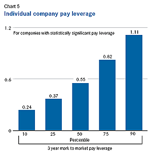There are wide variations in individual company pay leverage Plotting relative pay against relative performance for individual companies provides broadly similar results. The limited number of executives reported in the proxy and the lack of data available on business unit performance make it challenging to develop accurate pay leverage estimates for individual companies. Among 2,728 companies in the Execucomp database with at least one executive with three consecutive years of pay data, 1,413 have data for less than half of the 15 three-year periods ending in 1995-2009. Within this reduced sample of 1,315 companies, only 740 companies have pay leverage that is statistically significant. [17] The analysis below also limits the sample to top-three (instead of top-five) executives to reduce the likelihood of including business unit heads who might be compensated based on business unit performance.

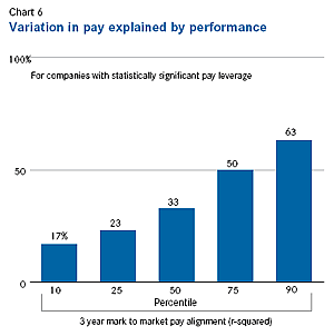Chart 5 shows that the median pay leverage of these 740 companies is 0.55. All but 26 of them have positive pay leverage, but less than 5 percent have pay leverage at or above the 1.4 pay leverage implied by the “pay percentile equals performance percentile” equation.

Chart 6 shows that relative performance explains 33 percent of the variation in relative pay for the median company with statistically significant pay leverage.

What Explains Differences in Pay Leverage?

There is widespread agreement that management compensation has three basic objectives: provide strong performance incentives, retain key talent, and limit shareholder cost.

Many companies believe those objectives can be achieved by combining a target competitive position—typically a 50th percentile pay—with a high percent of pay at risk. Given this common approach to achieving the basic objectives of executive compensation, one would expect that percent of pay at risk or percent of pay in deferred equity would largely explain differences in mark-to-market pay leverage. Surprisingly, however, this is not case.

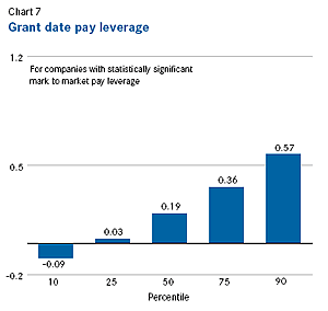
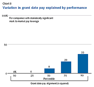Instead, a significant part of the variation in mark-to-market pay leverage is due to differences in grant-date pay leverage. Grant-date pay leverage is calculated using annual grant-date total compensation and relative TSR for the three years ending in the total compensation year; log relative pay is regressed on log relative performance, where relative pay is grant-date total compensation divided by the trendline grant-date total compensation for each executive’s position, industry and company revenue size. Grant-date pay leverage is considerably lower than mark-to-market pay leverage. Chart 7 shows that the median grant-date pay leverage of the 740 companies is 0.19—barely one-third of the median mark to market pay leverage. Consistent with this low leverage, performance explains only 8 percent of the variation in grant-date pay for the median company, as shown in Chart 8. However, the range in grant-date pay leverage is 75 percent of the range in mark-to-market pay leverage. The range in grant-date pay leverage from the 10th to the 90th percentile is 0.66, while the range in mark-to-market pay leverage from the 10th to the 90th percentile is 0.87.

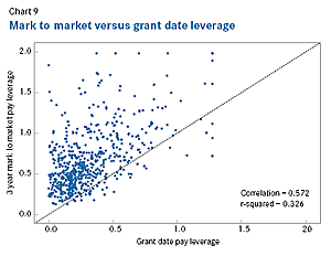Chart 9 shows that grant date pay leverage is lower than mark-to-market pay leverage, but explains 33 percent of the variation in mark-to-market pay leverage observed in companies with positive leverage. In this chart, mark-to-market pay leverage is on the vertical axis and grant-date pay leverage is on the horizontal axis, so mark-to-market pay leverage is greater than grant-date pay leverage for points above the main diagonal. All but a handful of companies are above the main diagonal, but the chart also shows that mark-to-market pay leverage is substantially correlated with grant-date pay leverage. Controlling for grant-date pay leverage, percent of pay at risk, percent of pay in equity and percent of pay in options all have a positive impact on mark-to-market pay leverage, but, in the aggregate, these at risk variables only explain another 3 percent of the variation in mark-to-market pay leverage. In a two-factor model using grant-date pay leverage and percent of pay at risk as explanatory variables, predicted mark-to-market pay leverage is equal to .161 + .830 x grant-date pay leverage + .386 x percent of pay at risk. This model implies that a .01 increase in grant-date pay leverage increases mark-to-market pay leverage by .008, while a 1 percentage-point increase in percent of pay at risk increases mark-to-market pay leverage by .004.

Assessing Pay-for-Performance: What a Director Can Do

To assess pay for performance, directors should set a tentative objective for incentive strength (i.e., mark-to-market pay leverage) and ask a series of questions:

• 1. What is the company’s mark-to-market pay leverage?
• 2. Has the company achieved the objective for incentive strength set by the board of directors?
• 3. If not, what is the company’s grant-date pay leverage? What is the company’s average percent of pay at risk?
• 4. Are the company’s grant-date pay leverage and average percent of pay at risk normally sufficient to achieve the directors’ target mark-to-market pay leverage?
• 5. If so, why do the company’s incentive plans fail to provide normal leverage?
• 6. If not, what is the combination of grant-date pay leverage and average percent of pay at risk required to achieve the directors’ target mark-to-market pay leverage?

The IBM example Assuming that the directors’ objective for mark–to-market pay leverage is 0.9 (above the 75th percentile, but well below the 1.4 leverage implied by the “pay percentile equals performance percentile” equation), we show how directors can address the six questions above using IBM as an example.

The dashed line in Chart 10 shows IBM’s pay leverage of 0.76. Pay leverage is the regression trendline relating log relative pay to log relative performance and pay leverage of 0.76 means that a 10 percent increase in relative shareholder wealth increases relative pay by 7.5 percent, on average. [18] If a company’s top executive received a fixed number of shares of stock each year (and no other pay), pay leverage would be 1.0 because 10 percent outperformance would increase pay by 10 percent. The solid line on the main diagonal shows pay leverage of 1.0.

The solid line on the main diagonal also shows where relative pay is equal to relative performance. If the plot points are predominantly above the solid line, relative pay is above average and the company has a strong retention incentive. Each plot point represents a three-year period for one executive. Dates with no suffix (e.g., “99”), denote the three-year period ending in that year for the CEO. Dates with a “b” or “c” suffix (e.g., “99b” or “02c”) denote the three-year period ending in that year for the #2 or #3 executive.

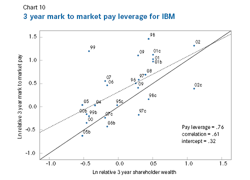
The correlation is a measure of how closely the individual points fit the pay leverage trendline. If all the points fall on an upward sloping line, the correlation will be 1.0 and all of the variation in pay will be attributable to performance. If the points are widely scattered around the line, the correlation will be close to zero. The correlation provides a partial measure of cost-efficiency. When it is close to 1.0, pay leverage is provided very efficiently because there is little pay that is unrelated to performance. Instead, when it is close to 0, pay leverage is provided very inefficiently. In some unusual cases, the correlation is negative and indicates that high relative pay is associated with low relative performance. A negative correlation is meaningful and appropriate in judging pay for performance—it is worse than a zero correlation between pay and performance.

Since IBM falls below our target mark-to-market pay leverage of 0.9, it is worth looking at whether its grant-date pay leverage and its average percent of pay at risk would normally achieve the target mark-to-market pay leverage. Chart 11 shows that IBM’s grant-date pay leverage is -0.05. Its average percent of pay at risk is 82 percent. Using the trendline above, average mark-to-market pay leverage for a company with IBM’s grant-date pay leverage and percent of pay at risk is .44. [19]

Two tentative conclusions can be drawn from this trendline model. First, it suggests that IBM’s incentive compensation is significantly more leveraged than average since its actual mark-to-market pay leverage is considerably higher than average for its grant-date pay leverage and percent of pay at risk.

Second, it suggests that an increase of 0.17 in IBM’s grant-date pay leverage would be sufficient to achieve our target mark-to-market pay leverage of 0.9. [20] An increase of 0.17 would raise IBM’s grant-date pay leverage from -0.05 to +0.12.

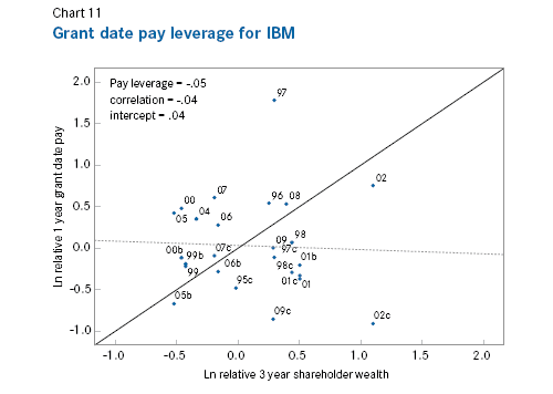
Since grant-date pay leverage of 0.12 is below the median grant-date pay leverage of 0.19, IBM could achieve target mark-to-market pay leverage of 0.9 with little departure from competitive practice. However, to achieve the mark-to-market pay leverage implied by the “pay percentile equals performance percentile” concept—that is, 1.4—IBM would need more radical changes in its compensation practices. The leverage model described in this report suggests that IBM would need to increase grant-date pay leverage by 0.77 to achieve this target. [21] This would increase its grant-date pay leverage from -0.05 to 0.72, a level that is well above the 90th percentile of current practice.

Conclusions

One key conclusion is that companies and directors need to measure pay leverage and set objectives for pay leverage. The “pay percentile equals performance percentile” concept is not a substitute for measuring and targeting pay leverage. It is impossible to use the concept to calibrate an incentive plan without understanding the pay leverage implied by “pay percentile equals performance percentile.” Moreover, many companies will find that the pay leverage implied by “pay percentile equals performance percentile” is far higher than they are comfortable with.

A second key conclusion is that measuring pay leverage requires substantial historical pay data. Companies need to calculate mark-to-market pay for an extended period. They need to calculate relative pay and relative performance and then run a pay-for-performance regression to get three key numbers: pay leverage, correlation, and the pay premium at industry average performance.

A third key conclusion is that companies have widely varied pay leverage. Pay leverage in the top quartile of companies is triple the pay leverage in the bottom quartile of companies. Directors need to consider optimal pay leverage for their company. It’s unlikely that a single answer e.g., the pay leverage implied by “pay percentile equals performance percentile,” will be optimal for all companies.

A fourth key conclusion is that a high percent of pay at risk is not the simple answer to strong incentives. A high percent of pay at risk contributes to mark-to-market pay leverage, but the pay leverage of grant-date pay is more important. A target competitive position—based only on size—and a target percent of pay at risk may be adequate to achieve the company’s objectives for incentive strength, retention risk, and shareholder cost, but directors should consider whether there are more efficient alternatives that tie the company’s target compensation levels to size and performance.

Endnotes

[1] Procter & Gamble proxy statement, filed Aug. 27, 2010, p. 24 (www.pg.com).
(go back)

[2] ISS Governance Services “2008 U.S. Proxy Voting Guidelines Summary,” December 17, 2007, 30.
(go back)

[3] Dow Chemical proxy statement, filed March 31, 2010, p. 20 (www.dow.com).
(go back)

[4] CSX Corporation 2010 proxy statement, filed March 24, 2010, p. 25, (www.csx.com).
(go back)

[5] The Conference Board, “Final Report of the Task Force on Executive Compensation,” 2009, p. 18 (www.conference-board.org/pdf_free/ExecCompensation2009.pdf).
(go back)

[6] Pay Governance SEC Comment Letter, September 14, 2010 (www.sec.gov/comments/df-title-ix/executive-compensation/executivecompensation-11.pdf).
(go back)

[7] For the years 2006–2009, the Summary Compensation Table reflected the accounting allocations used for financial reporting. Beginning in 2010, the Table includes the full expected value of equity compensation grants made in the year.
(go back)

[8] The dependent variable in each regression is the natural log of three-year mark to market pay; the independent variables are mean log pay for the executive’s position or rank (i.e., CEO, rank #2, …, rank #5) and the difference between the natural log of company revenue for the executive and the mean log company revenue for the executive’s position or pay rank.
(go back)

[9] The first three-year period is 1993–1995, there are 15 three-year periods ending in 1995-2009 and 24 industry groups, 15 x 24 = 360.
(go back)

[10] See, for example, Arch Patton, “Building on the Executive Compensation Survey,” Harvard Business Review, Vol. 33, 3, May/June 1955.
(go back)

[11] For example, in Chart 1, the percent change from the 25th percentile to the 50th percentile is +60% (= 101%/63% – 1) and the percentage change from the 50th percentile to the 75th percentile is +65% (= 167%/101%), for a total of +125%, but the percent change from the 25th percentile to the 75th percentile is +165% (= 167%/63% -1).
(go back)

[12] To convert the log differences to percentage differences, we need to use the antilog or exponential function. Exp(-0.45)-1 = 0.638 – 1 = -.362. Exp(+0.39)-1 =.477.
(go back)

[13] The log measure of relative performance is ln(relative shareholder wealth) = ln((1+TSR)/(1 + industry TSR)). TSR is not annualized.
(go back)

[14] This is equal to the ratio of the change in log relative pay to the change in log relative shareholder wealth. Pay leverage at percentile p = [ln(relative pay_p+1) – ln(relative pay_p) ]/[ln(relative shareholder wealth_p+1) – ln(relative shareholder wealth_p)] = ln(relative pay_p+1/ relative pay_p)/ln(relative shareholder wealth_p/relative shareholder wealth_p).
(go back)

[15] Relative shareholder wealth will have exactly zero correlation with the industry TSR only when the industry “beta” is 1.00, i.e., when a regression of ln(1 + actual TSR) on ln(1 + industry TSR) has a slope of exactly 1.00.
(go back)

[16] Target leverage of 0.80 implies that ln([vest_p+1/vest_p] x [stock_p+1/ stock_p])/ln(stock_p+1/stock_p) = 0.80; then ln([vest_p+1/vest_p] x [stock_p+1/ stock_p] = 0.80 x ln(stock_p+1/stock_p);[vest_p+1/vest_p] x [stock_p+1/ stock_p] = (stock_p+1/stock_p)0.80; and finally, [vest_p+1/vest_p] = (stock_p+1/ stock_p)^-0.20.
(go back)

[17] Subtracting the 1,413 companies with less than eight data years from the total sample leaves 1,315 = 2,728 – 1,413.
(go back)

[18] Ln relative pay = constant + 0.76 x ln relative shareholder wealth implies relative pay = exp(constant) x relative shareholder wealth^0.76. A 10 percent increase in relative shareholder wealth is equivalent to multiplying by 1.1^0.76 and 1.1^0.76 – 1 = .075.
(go back)

[19] The trendline is mark-to-market pay leverage = 0.161 + (0.830 x grant-date pay leverage) + (.386 x percent of pay risk). This gives a predicted value for IBM of 0.161 + (.830 x -0.05) + (.386 x .82) = 0.436.
(go back)

[20] (Target pay leverage – actual pay leverage)/grant-date pay leverage coefficient = required increase in grant-date pay leverage. (.9 – .76)/.830 = 0.17.
(go back)

[21] Dividing the needed increase in mark-to-market pay leverage by the coefficient of grant date pay leverage, we get a required increase of 0.77 in grant date pay leverage, 0.77 = (1.4 – .76)/.830.
(go back)