 Print
PrintBen Burney is a Senior Advisor at Exequity, LLP. This post is based on his Exequity memorandum.
When you hear the words “Monte Carlo simulation,” do you:
- Scream;
- Pack your suitcase—Mediterranean vacation! (Simulation? Nah!); or
- Ponder the link between 19th century botany and modern valuation techniques? If you chose a) and would rather b), read this post to c).
For management teams and compensation committees, Monte Carlo simulations are often only marginally understood. Trying to figure out what is going on makes some want to scream (or pack their suitcases). These decision makers may know that Monte Carlo simulations are used to value awards with market conditions (like relative total shareholder return (RTSR)), but not how it works or why values are high or low.
Reviewing Monte Carlo simulation results prepared by valuation firms is not always helpful either—the materials are often filled with statistical jargon. The implication is clear: This analysis is really, really complicated.
And so, important decisions may be made in a vacuum. Designs may be based solely on market practices reported in surveys (such as Exequity’s) or peer groups, leading to the approval of design parameters without a full understanding of the implications of these choices. Key questions may be overlooked, such as:
- Do our TSR awards align with our compensation philosophy? Pay mix?
- Is it possible to estimate the likelihood of TSR awards paying out?
- How does design impact the Monte Carlo values? And why?
- Can an award be designed to improve the relationship between the disclosed grant value of the award and the ultimate earned value?
- Should we denominate TSR awards using Monte Carlo values or stock price?
This post offers a plain-English guide to the Monte Carlo simulation technique. By understanding how simulations “predict the future,” we can better understand the implications of compensation design decisions. Our goal is to help decision makers understand how the technique works, why the Monte Carlo values may be high (or low), and the impact of design choices on valuation outcomes.
[Next], we describe market conditions and how companies tend to think about Monte Carlo values. Then, we explore what is behind Monte Carlo and how design choices impact values.
What Is a Market Condition?
A market condition is a vesting condition based on stock price performance. An example of an award with a market condition would be one that compares a company’s stock price performance to that of a peer group. ASC Topic 718 requires that awards with market conditions be valued using a valuation technique that considers the possible outcomes of the award. Monte Carlo simulations formulaically model the spectrum of probable outcomes, satisfying the Topic 718 requirement.
How Do Companies Use Monte Carlo Values?
In our experience, there tend to be two general approaches to using Monte Carlo values. Some companies use these values for accounting purposes only, others for accounting and award sizing. The reason that this distinction is important is that the Monte Carlo value of an award often is higher than the face value of the shares underlying the award. Therefore, if an employee’s award is determined by dividing the intended grant value by the Monte Carlo value, fewer shares will be included in the award.
Approach #1: Monte Carlo Values Are Just for Accounting
When Monte Carlo values are used for accounting purposes only, the sense is that the Monte Carlo values (accounting costs) “are what they are.” The company does not believe the accounting costs should impact how awards are denominated. Companies recognize that by adopting market-based awards, they need to value them in accordance with Topic 718 (i.e., they need to “run a Monte Carlo”). They design the award parameters in line with what they feel are the right design inputs, possibly giving less weight in their decisions to accounting costs. This can lead to disparities between the accounting cost for the market-based award and the price used to denominate the award. Some companies are comfortable with this and do not view the accounting costs as being preferable to their standard denomination method.
This is particularly true when the Monte Carlo value significantly exceeds the grant-date stock price because many companies feel that participants should not be penalized (i.e., awarded fewer shares) by virtue of the company’s choice to use a market condition versus a financial condition.
Approach #2: Monte Carlo Values Should Be Used for Denominating Awards and Accounting
The other school of thought is to denominate awards using the Monte Carlo value. In this school of thought, the use of Monte Carlo values for denominating market-conditioned awards is roughly equivalent to the use of Black-Scholes values for denominating stock options. Differences between the Monte Carlo value and the stock price on the grant date can lead to disparities between the number of shares granted using the Monte Carlo value relative to what might have been granted using the stock price at grant. However, under this methodology, the “intended” grant value approximates the disclosed value.
Example: To demonstrate, assume a company wishes to grant $1,000 in RTSR awards. The stock price at grant is $20 and the Monte Carlo value at grant is $25. Under the first school of thought, where the accounting costs are less important, 50 shares would be granted. The accounting cost is $1,250 ($25 x 50 shares), but the “intended” compensation value is $1,000 ($20 x 50 shares). Under the second school of thought, only 40 shares are granted. The accounting cost and “intended” grant value is $1,000 ($25 x 40 shares), though the intrinsic value of the 40 shares granted is $800 ($20 x 40 shares).
Which Method Is Best?
Exequity does not maintain a position on what is “right” for all companies. There are pros and cons to both approaches that need to be reconciled with each company’s compensation philosophy. Management teams and compensation committees should be informed of potential differences between the alternative methods, and why the differences exist. Companies may also consider discussing these differences in their disclosures. Armed with this knowledge and a better understanding of how the process works, we hope companies are then better prepared to think strategically about their market-based awards.
The Monte Carlo Simulation Technique
The Monte Carlo simulation technique employs a three-step process:
- Step #1: Gather and analyze historical market information (daily price returns) for the company (and peers if relative performance is measured).
- Step #2: Generate simulated TSRs for the company (and peers, as applicable). This process is an iterative process conducted thousands of times, with each iteration representing a probable
- Step #3: Assess sponsor performance based on defined parameters, and assign payouts for each iteration of the simulation; the Monte Carlo value is the present value of the average payout
Below we unpack what happens at each of these process steps and how peer group and design choices impact valuation outcomes.
Gathering Model Inputs Using Historical Returns
The first step in the process is to gather historical returns (daily price changes) for the company, and when RTSR is measured, for peer companies. The period corresponding to the remaining performance period from the date of grant defines the measurement period. The data gathered is used to calculate how the stock(s) analyzed may be expected to perform in the future, as defined by stock price volatility and, if applicable, stock price correlations. We will explain the importance of each in more detail over the following sections, but first it is important to define these terms.
- Volatility represents the magnitude of stock price movements. [1] High-volatility stocks experience larger day-to-day price movements than low-volatility
- Correlation measures the degree to which two stocks move together and applies to relative performance plans (e.g., RTSR). Highly correlated stocks move more in tandem with one another, while poorly correlated stocks do not. Correlations range from 1.00 (perfect correlation) to -1.00 (perfect inverse correlation).
How Future Stock Prices Are Simulated: “Geometric Brownian Motion With a Drift”
If there is a “secret formula” in the Monte Carlo simulation technique, it is the development of simulated stock prices. How is it done? The “Monte Carlo” aspect of this overall process simply refers to what is, in essence, “rolling of the dice” thousands of times. [2] Monte Carlo techniques can be applied to myriad scenarios involving forecasting or predictive modeling. For awards with market conditions, simulated future stock prices are defined using a specific formula, described below, with one of the inputs varying based on each “roll of the dice,” i.e., the Monte Carlo simulation technique.
The formula used to estimate future stock prices was developed based on an observed process called Brownian Motion. This process is named after Robert Brown, a 19th century botanist who observed the seemingly random movements of pollen particles in a fluid under a microscope. Over the following decades and into the 20th century, mathematicians and scientists developed ways of formulaically describing random movements of particles, atoms, and eventually in financial theory to describe the movements of stock prices. Today, the generally accepted method for simulating stock price paths is using a formula often referred to as Geometric Brownian Motion with a Drift. [3] The “Geometric Brownian Motion” portion of this formula refers to the random movements of the observed stock prices (pollen particles). The “drift” refers to constant forward motion, i.e., the passage of time. It can be thought of as a “breeze,” as though pollen particles are moving through the air over time assuming a constant wind speed. In other words, there are random movements mixing with a constant force. Some particles fly high into the sky (e.g., high TSR), some fall to the ground (e.g., low TSR), and some end up somewhere in between. We will refer to Geometric Brownian Motion with a Drift as GBM going forward.
Defining GBM
The GBM formula used to develop simulated stock prices for the company and each peer company is displayed below. This formula may bring back nightmares from math or statistics classes for some readers. We sympathize. We also seek to demonstrate there is no “secret formula.” Except for the random variable, “Z” (the “roll of the dice”), the inputs to this formula are fixed and based on historical market information gathered from the first step in the process. The GBM formula is:

The definitions for each of the variables in this formula are:
- ST: Simulated future stock price.
- S0: Beginning stock price (e.g., as of the grant date).
- e: The mathematical constant e (~2.72, i.e., the base of the natural logarithm).
- Rf: The risk-free interest rate based on zero-coupon U.S. Treasuries (the “drift”).
- d: The dividend yield (if applicable).
- σ: Annual volatility.
- T: The term of the award, from the grant date to the end of the applicable period.
- Z: Normally distributed random variable (Z-score); for simplicity, one can think of “Z” as a random number that changes for each simulation. [4]
Outputs of a Monte Carlo Simulation Using GBM
What does a simulation using this formula produce? A range of probable future returns (TSRs—change in stock price plus dividends), both negative and positive. For demonstration purposes, the graphic below depicts five simulated stock price “paths” of a single stock over three years of simulated daily trading activity, with each daily change defined using the GBM formula described above. Over each simulated trading day, the only variable which changes is the Z, which is driven by a random number generator. For relative performance awards, these generated random variables are transformed to be correlated with each other (described later). The example below displays five TSR paths for a single stock. One might even think of each stock price path as pollen floating in the breeze.
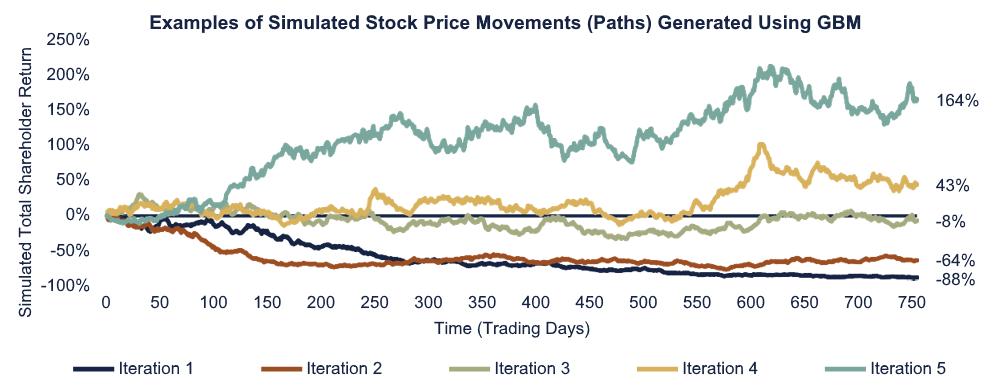
The Risk-Neutral Simulation Framework
Simulations are conducted in what is called a “risk-neutral” framework. This means the average of all the returns generated is equivalent to the risk-free rate (e.g., U.S. Treasuries). The risk-free rate is what is referred to as the “drift” (recall the constant breeze carrying pollen particles through the air). For example, assuming a 3% annual interest rate (pollen moving at a 3% “breeze”), the average of the simulated annual TSRs over the period is also 3%. In the example above, the interest rate is set at 3% and the average return of the five iterations is ~9% over the three-year period, equivalent to what a 3% annual return would otherwise generate over three years. The reason for conducting simulations in a risk-neutral framework is to isolate the impact of the market condition on the value of the award, considering the time value of money. [5]
Estimating the Value of Market-Conditioned Awards
Assuming these five simulations presented above are representative of a full simulation, and further assuming a grant price of $20 and a dividend yield of 1%, the table below presents the simulated values, their corresponding present values, hypothetical payouts, and finally, the fair value of the award. This is the general process by which fair values are calculated, from the generation of simulated results to the Monte Carlo value ascribed to the award.
Here is the basic process for calculating the Monte Carlo value in stepwise order, moving from the top of the table down (Step 1, Step 2, etc., with each step in the list corresponding with a row in the table):
- Step 1: Simulate TSRs—Simulated results (TSRs) are calculated. Five iterations are shown.
- Step 2: Ending Value—The average ending value of the award is $21.89 (including dividends), which is roughly equivalent to $20 grown at 3% per year for three years.
- Step 3: Present Value—The values resulting from each iteration are discounted to present at the risk- free rate of 3% (i.e., the present value). This results in an average value of $20 (equal to the granted value).
- Step 4: Dividend Discount—Assuming award holders do not have rights to receive dividends (i.e., dividends are not accrued, even for vested shares), the values are discounted (i.e., dividend discount), resulting in an average value of $19.41.
- Step 5: Payout Factor—The payout factors resulting from simulated performance results are applied, further modifying potential payments under each iteration. [6]
- Step 6: Monte Carlo Value—The Monte Carlo value [7] of the hypothetical award is the average of the final payout value for each iteration. In this hypothetical scenario, it is $27.73, 139% of the grant price of $20.
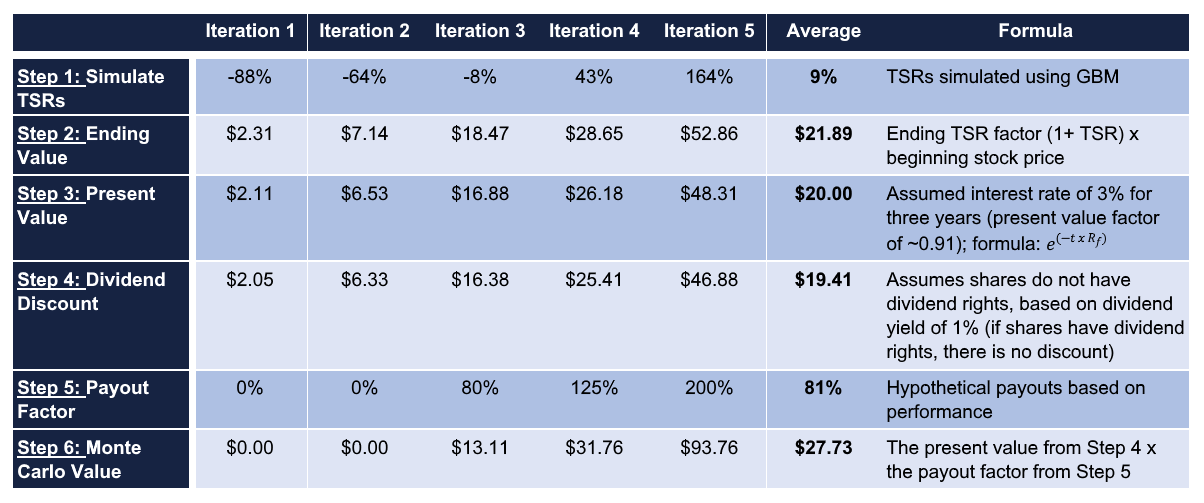
The Monte Carlo value is the present value of the average payout: $27.73.
Factors Impacting Monte Carlo Simulation Results
This next section describes how variations in several key factors impact the Monte Carlo values of awards. The factors explored are volatility, correlation (for RTSR awards), and leverage (payout factors) in award design.
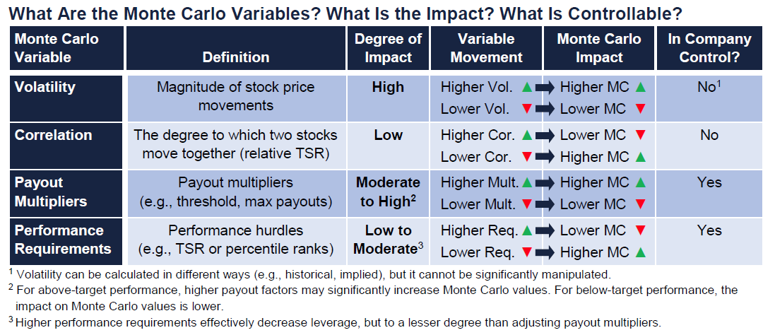
How Do the Key Variables Impact Monte Carlo Values?
The influence of these factors on Monte Carlo values, detailed further herein, is summarized below:
- Volatility: In most cases, Monte Carlo values of awards for higher-volatility companies will exceed those for lower-volatility companies.
- When performance requirements are satisfied, ending values can be very high and may possibly be multiplied by a payout factor (e.g., 1.5x the targeted number of shares), which further increases the Monte Carlo value.
- The increased payout values for these positive TSR iterations more than not offset the iterations where no payout occurs, i.e., the fair value is more likely to exceed the grant price of the shares underlying the award.
- Correlation (relative performance): For RTSR and relative performance awards, higher correlations between peers slightly dampen Monte Carlo values.
- Higher correlations reduce the peer group “noise.”
- Reduced “noise” means that when the sponsor company’s TSR is high, the other peer company TSRs are also more likely to be high, which may result in lower payout multipliers
- Increased correlation can slightly reduce Monte Carlo values.
- Design Leverage: Design leverage refers to the pay-for-performance relationship in the award design. Higher payout factors (e.g., 200% of target versus 125%) will increase Monte Carlo values; high payout factors for higher-volatility stocks result in very high Monte Carlo values.
- Higher payout factors for higher-volatility companies will have significantly higher Monte Carlo values than the same payout factors for low-volatility companies.
- Design leverage is the variable most within a company’s control for managing accounting expense (and grant values reported in the proxy statement).
What Is Volatility? How Does It Impact Monte Carlo Values?
Volatility represents the magnitude of stock price movements. High-volatility stocks experience larger price movements—higher or lower—than low-volatility stocks. High-volatility stocks carry a greater downside risk, but also the possibility of higher returns. Low-volatility stocks offer lower downside risk, but less upside. For demonstration purposes, the graphic below depicts the range of three-year expected returns for three hypothetical assets. The range of returns represented is between the 0.5th percentile (extremely low return) to the 99.5th percentile (extremely high return). [8] The three asset volatilities are:
- 13%, the approximate volatility of the S&P 500 Composite Index.
- 25%, approximately the average volatility of an individual S&P 500 stock.
- 50%, a hypothetical high-volatility stock.
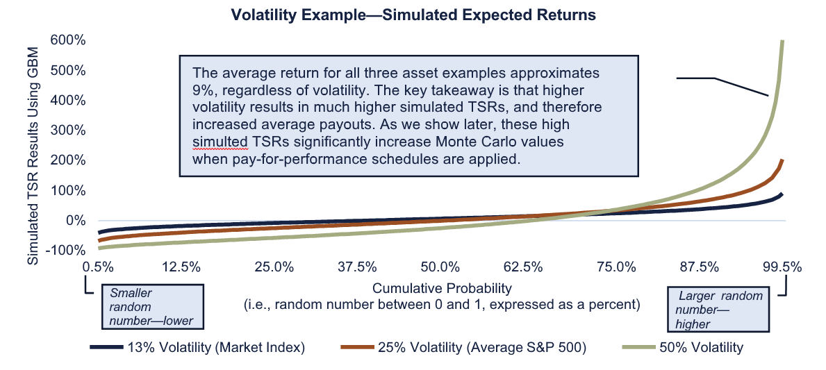
Additional detail on the range of results is provided in the table below:
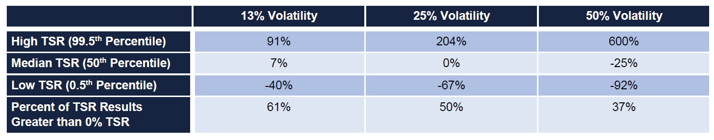
In this example, the low-volatility stock is more likely to generate positive returns (61% of the time above 0%) but offers limited upside; the high volatility stock generates positive returns only 37% of the time but is more likely to appreciate significantly. Due to the possibility of significant appreciation, the Monte Carlo value for a company with high volatility is typically greater than for a low-volatility company.
What Is Correlation? How Does It Impact Monte Carlo Values?
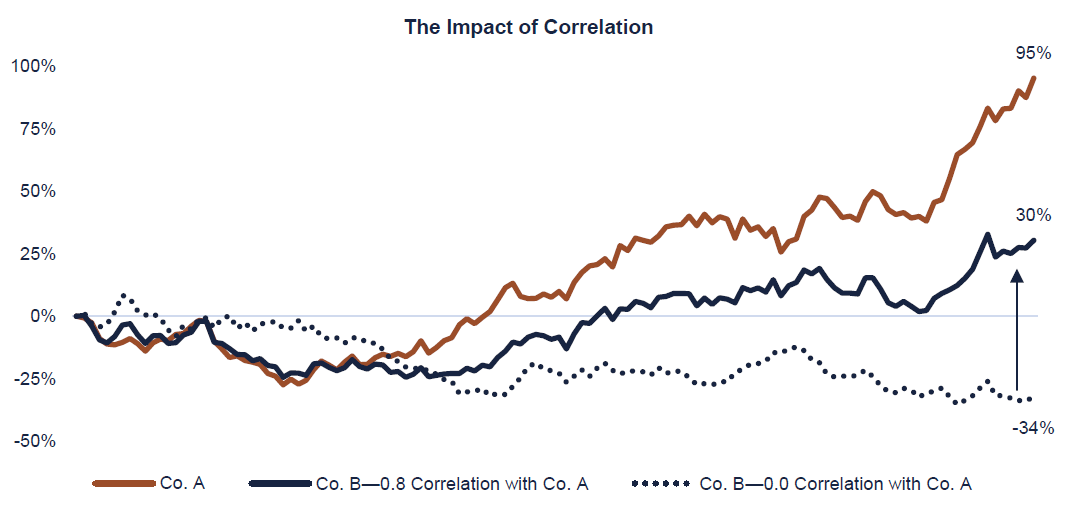
Correlation measures the degree to which two stocks move together. Highly correlated stocks move more in tandem than poorly correlated stocks. Correlations range from 1.00 (perfect correlation) to -1.00 (perfect inverse correlation). In a Monte Carlo simulation for valuing RTSR awards, the impact of correlation is applied in each iteration by modifying the “Z” (random number) variable at the end of the formula shown above. This is often done through a mathematical transformation process. [9] When random numbers are generated to develop simulated returns, this process modifies the series of random numbers to make them correlated.
The chart below displays TSR paths for two stocks before and after incorporating the impact of correlation. [10] The dotted blue line represents a simulated path for Company B, prior to adjusting for any correlation with Company A, i.e., the initial assumed correlation between Company A and Company B is 0.0 (no correlation). [11] In the example, the initial path of Company B results in -34% TSR; Company A’s path results in 95% TSR. Note that the day-to-day difference between the two is purely chance. Now, assume the correlation between these two companies is 0.8 (a very high correlation). This means these two companies have moved almost in tandem historically, and they would be expected to move similarly in the simulation. The incorporation of correlation is performed through the transformation process. Once the impact of the correlation between Company A and Company B is applied, Company B’s day-to-day movements, shown in the solid blue line, align better with Company A; this impacts Company B’s overall trajectory in this iteration as well, from -34% +30% TSR.
In a Monte Carlo simulation, higher correlations will slightly reduce the Monte Carlo value. The reason is that projected relative outperformance for the sponsor company may be less than if correlations were low, which lowers the projected payout multipliers. Lower projected payouts reduce the Monte Carlo value.
How Does Incentive Design (Leverage) Impact Monte Carlo Values?
In this section, we describe how leverage in the incentive design can impact Monte Carlo values. Leverage refers to the payouts corresponding with specified levels of performance. A common design for RTSR plans is a structure where certain percentile ranks versus a peer group correspond with specified payout multipliers. Here is a rather typical RTSR design:
| Performance Level | Percentile Rank vs. Peer Group | Payout as a Percent of Target |
|---|---|---|
| Below Threshold | Less than 25th Percentile | 0% |
| Threshold | 25th Percentile | 50% |
| Target | 50th Percentile | 100% |
| Maximum | 75th Percentile or Greater | 200% |
For example, assume an employee is granted 50 shares at a stock price of $20 (an intrinsic value of $1,000 at grant). Under this structure, if RTSR performance at the end of the performance period exceeds the 75th percentile, the employee would receive 200% of the shares granted, 100 shares. If the value at vesting is $40, the employee’s vesting value would be $4,000. If performance falls below the 25th percentile, no payout would occur, regardless of the ending stock price. For all companies, increased leverage (e.g., payout multiplier) [12] results in higher potential payouts, which increases the average payout (and the Monte Carlo value). Decreased leverage lowers the average payout.
Using the table above as an example illustrates the impact of adjusting the payout multipliers and performance requirements. Reducing the iterations with 125% and 200% payouts reduces the average from $27.73 to $22.40, a 19% reduction. Making the threshold payout higher (e.g., minimum payout of 50%) increases the average from $22.40 to $23.24, a 5% increase. This demonstrates that higher payout factors (at high performance) have a more significant impact on Monte Carlo values than easing requirements at low performance levels. The reason is that at high performance, the ending values are higher, pulling the average up more than lower payouts for low performance push the average down.

1 The same value as displayed in the “Dividend Discount” row in the table above.
What Is the Combined Impact of Volatility, Correlation, and Design?
What is the combined impact of these three variables (correlation, volatility, leverage) on Monte Carlo values? For demonstration purposes, we ran Monte Carlo simulations for four peer groups based on varying inputs. Across the four scenarios, the sponsor company and the peers have high correlations (0.50 each) or low correlations (0.20 each) and either high volatility (50% each) or low volatility (20% each). As a reminder, higher correlations and lower volatilities each result in lower fair values generated by Monte Carlo simulations. We then apply maximum payout factors of 200%, 150%, and 125%. All values are based on a $20 grant price.
| 200% Max Payout | 150% Max Payout | 125% Max Payout | ||||
|---|---|---|---|---|---|---|
| 20% Volatility (Low) | 50% Volatility (High) | 20% Volatility (Low) | 50% Volatility (High) | 20% Volatility (Low) | 50% Volatility (High) | |
| 0.50 Correlation (High) | $24.50 | $29.25 | $19.75 | $23.00 | $17.25 | $20.00 |
| 0.20 Correlation (Low) | $25.50 | $31.00 | $20.25 | $24.25 | $17.75 | $21.00 |
Note: In this example, threshold performance is the 25th percentile (50% payout) and maximum is the 75th percentile (125%/150%/200% payout). All figures rounded to the nearest $0.25.
Why Are the Monte Carlo Values So High? What Can Be Done?
The most common cause of high Monte Carlo values is a higher volatility or a combination of higher volatility with higher payout factors (e.g., 200%). In most cases, volatility cannot be “managed” or otherwise manipulated. [13] The most effective, but oftentimes least desirable, ways to reduce the Monte Carlo value in these situations are first to reduce payouts and second to increase performance targets. When awards are denominated based on the Monte Carlo value, reducing leverage results in granting more shares, which may help assuage (some) participants that this is not a “takeaway.”
The peer group is another variable within the company’s control for RTSR plans. Peer groups consisting of companies more like the sponsor may (not always) reduce Monte Carlo values, via increased correlation. (Monte Carlo values aside, a highly correlated peer group is preferable regardless of the valuation as it enhances the pay-for-performance relationship, lessening the impact of extraneous forces on relative performance.)
While there are other reasons for Monte Carlo values being high and other methods for reducing these values, some solutions involve adding more layers of complexity. Examples include holding periods and capping payouts at a certain dollar value. We suggest making sure stakeholders understand the rationale for additional layers of complexity to market-conditioned awards. Incentives can lose their impact when participants do not understand them.
Final Thoughts
Exequity’s experience is that Monte Carlo simulations are not generally well understood. In our view, decision makers in management teams and on boards can benefit from a more thorough understanding of how Monte Carlo values are generated. In cases where awards are being determined based on Monte Carlo values, understanding the meaningful variables and the impact of incentive design on grant values is important in ensuring that the awards deliver the intended motivation and value. We hope this Client Briefing helps decision makers ask and answer important questions in pursuit of improved award designs.
Quick Guide to the Impact of Key Variables Used in Monte Carlo Simulations
Why Are the Monte Carlo Values So High? What Can Be Done?
The most common cause of high Monte Carlo values is high volatility, or a combination of high volatility and higher payout factors (e.g., 200% or higher). Methods to reduce the Monte Carlo value are:
- High Impact: Reduce Payout Factors, e.g., instead of 200% maximum payout, use 150%.
- Leverage above target performance has the greatest impact; reducing leverage may not be desirable, but it is the most effective means of reducing the Monte Carlo value. [14]
- Reducing payouts for low performance has less impact than reducing payouts about target.
- Moderate to High Impact: Increase Performance Requirements, e.g., instead of max at 75th percentile, increase to the 90th percentile.
- Increasing threshold performance requirement (e.g., from 25th percentile to 35th) has less impact than increasing performance requirements about target.
- Low Impact: Peer Group May Be Adjusted to be more comparable to the sponsor company.
- Peer group selection can impact Monte Carlo values, but not always in a material way; however, use of highly correlated peers lessens the impact of extraneous forces on relative performance.
- Selecting the right peer group is important for philosophical reasons; it also tells participants and investors the types of companies the company seeks to outperform (usually industry competitors).
Endnotes
1In technical terms, volatility is the annualized standard deviation of lognormal daily stock price returns.(go back)
2The Monte Carlo simulation is named in homage of the gambling mecca, the Monte Carlo casino, in the Principality of Monaco in Western Europe.(go back)
3This simplified background information glosses over numerous mathematicians, scientists, and others who contributed to developing the statistical theories and processes underlying the Monte Carlo simulation technique using Geometric Brownian Motion (used to estimate values of market-conditioned awards). The mathematics behind the development of this formula are very complicated and outside the scope of this Client Briefing. We also note that professors Fischer Black, Myron Scholes, and Robert Merton developed their method for valuing stock options, now commonly known as the Black-Scholes formula, based on Geometric Brownian Motion principles.(go back)
4To define the Z variable (the “roll of the dice”), a random number generator defines values between 0 and 1 (cumulative probability), which are converted into the normal distribution (mean of 0 standard deviation of 1); this is a standard statistical process. For example, for the random number 0.25, the Z value is -0.67; 0.75 has a Z value of 0.67; 0.99 has a Z value of 2.33. Further details on the derivation and nature of the normal distribution are beyond the scope of this Client Briefing.(go back)
5The basic principle of the time value of money is that $1.00 today is worth more than $1.00 tomorrow, because money can earn interest. For example, $1.00 today is worth $1.03 in one year at a 3% risk-free rate. The “present value” of $1.03 (i.e., from one year from now to today) is $1.00.(go back)
6For RTSR awards, simulated sponsor performance is measured relative to the simulated performance of the peers. Other conditions may include a negative TSR cap (e.g., maximum payout at target if TSR is negative).(go back)
7While we use the colloquial “Monte Carlo value,” the more technical term is “estimated fair value.” Estimated fair value is commonly used in valuation documents. For our purposes here, the terms are interchangeable.(go back)
8For this example, the endpoints are 0.005 and 0.995, ~2.6 standard deviations above/below the mean. This means 0.5% of possible instances are higher or lower at each end of the spectrum (these 0.5% ends are not displayed).(go back)
9The typical process for transforming uncorrelated random numbers into correlated random numbers is called Cholesky Decomposition. The mechanics of this process are beyond the scope of this Client Briefing.(go back)
10In a two-company example, only one stock price path needs to be modified. In this example, the volatility for each company is the same.(go back)
11Over the period, Company B’s trajectory is lower, but that is simply due to the random nature of price movements over time in this iteration. These particular paths were chosen as they demonstrate the impact of correlation.(go back)
12Increased leverage can occur with higher multipliers or lower performance requirements. Decreased leverage can come from lower payouts or higher performance requirements.(go back)
13Some companies use implied volatility, which is based on the trading of stock options, in their volatility calculations.(go back)
14Note, when the Monte Carlo value is used to denominate the award, the negative effect of a reduced maximum is partially offset because more shares are granted (each share carries a lower Monte Carlo grant value).(go back)